Building A Bayesian Prediction Model For NCAA Hockey

How machine learning, junior league translation factors, and Bayesian inference combine to forecast every roster in college hockey

How many points will a player produce next season? How will a freshmen goaltender perform? How does a projected roster stack up?

With college hockey gaining increasing popularity, I wanted to introduce something new. Something useful that can help us answer these questions. Rarely is there a systematic, reproducible answer that covers every player on every roster at this level—freshmen, veterans, transfers, and goalies alike.

That is what I have spent the last several months building.

Before projecting anything, there is a more important question to answer first: does any of this actually work?

Before pointing the model at 2026-27 rosters, the entire framework was built and validated using 2024-25 end-of-season data to project 2025-26 production. Those results were then checked against what players actually did. Every skater. Every goalie.

That audit validated the translation logic, the age curves, and the model framework before a single future projection was generated.

The Junior Translation

A 70-point junior season sounds impressive, but 70 points in the USHL is not the same as 70 points in the OHL, which is not the same as 70 points in the NCAA. Context matters.

Before any junior player enters the model, his production is run through a league-specific translation formula. As I’ve noted in previous studies, scoring rates translate differently depending on the source league.

How CHL Scoring Rates Translated To NCAA During 2025-26 Season

Since those initial studies, I have received numerous inquiries regarding NAHL data. Unfortunately, my data source, InStat, lacks recent data for the league. To bridge this, I used 2022-23 NAHL data, observed how those rates translated to the NCAA for 2023-24, and incorporated those findings into my model.

Of note, until I have more of a sample size to work with, ECHL players have been omitted from the model.

For returning NCAA players, the translation step is skipped entirely. Their college production history becomes the direct input, adjusted forward based on role and development arc. The effects of the transfer portal were also factored into these projections.

The Age Development Curve

An 18-year-old freshman and a 21-year-old junior are fundamentally different prospects; treating them identically would be a modeling error. After studying four seasons of NCAA data on how production evolves with age, a clear pattern emerged: forwards peak early, defensemen peak late.

The 18-to-19 transition is when most skilled forwards make their biggest offensive jump. By 20 or 21, that spike has usually already occurred; future gains come from expanded roles, not raw development. Defensemen work on a longer runway. Offensive upside at the blue line often does not fully emerge until a player is logging top-four minutes and regular power-play time as an upperclassman.

Both the player’s age at the start of the season and its squared value are included as model features, allowing the framework to capture the nonlinear shape of that development curve rather than assuming a straight-line progression.

The transfer portal adds another layer. A young forward moving to a stronger program or leaving for more playing time can see an immediate scoring jump, while a young defenseman changing systems often struggles before settling in. By the time a player crosses age 21, those effects largely disappear, as the data revealed that experienced transfers generally carry their production with them directly into a new situation.

What the Box Score Misses

Points alone do not paint the full picture.

To measure actual efficiency, the model considers additional average-per-game data, ensuring a fourth-liner producing in limited minutes receives a fair comparison against a top-line forward playing 22 minutes a night.

The model incorporates six underlying rate metrics that capture what the box score cannot: expected goals, slot passes, puck touches, scoring chances, takeaways, and zone entries. Rounding out the twelve features are raw PPG from the prior season, age, age squared, transfer status, CORSI percentage, and puck battles won percentage.

Together, these inputs form the model’s baseline vision.

How the Skater Model Works

Once features are cleaned, translated, and rate-scaled, they are processed through a hierarchical Bayesian regression model that accounts for the environment in which each player competes.

The core idea is that a point scored in the Big Ten and a point scored in the AHA do not carry the same weight. Therefore, conference strength is baked into the model as a structural component.

For incoming freshmen with no NCAA track record, the model applies a conservative approach to the adjustment required to compete at this level. First-year players are volatile by nature, and a model that overpromises on freshmen is a model that cannot be trusted.

Furthermore, the Bayesian approach produces something a traditional model cannot: uncertainty. Every skater is assigned not just a projected PPG, but a realistic range of outcomes, reflecting the model’s confidence in that specific projection.

What About Goalies?

Projecting goaltenders means throwing the points framework out entirely. Goalies don’t score. So what do you measure?

The answer is GSAx, or Goals Saved Above Expected). Rather than counting goals allowed, we measure how many goals a goalie allowed compared to the quality of shots he faced.

The goalie model uses a two-stage approach. First, a Random Forest is trained on 2025-26 NCAA goaltender data, using age, save percentage, and league translation factors, to produce a “prior” projection for each goalie in the 2026-27 pool. Then, a Bayesian update combines that prior with the goalie’s observed performance, weighted by ice time. The result balances the model’s expectation with the goalie’s actual show of form.

This estimate is then scaled into a 0–10 rating centered at 5.0, where anything above 5.0 implies a strong goaltender and anything below indicates an underperformer. Conference strength multipliers are applied here as well.

For junior goalies entering the college game, I applied a similar translation logic to observe how junior goaltending rates convert to the NCAA level.

(If you’d like to see a separate write-up on the goaltending rate translations, I’d be happy to share that. If you’re more interested in the TL;DR version: USHL, OHL: Good, WHL: Stable, QMJHL/BCHL: Adjustments Needed)

What the Audit Actually Found

This is where the model earns its credibility.

For skaters, the results were strong. Across more than 1,400 players, the model explained 79% of scoring variance league-wide. Put plainly: nearly four-fifths of the difference in how players scored across an entire season was captured by factors the model accounted for before the puck dropped. The linear correlation between projected tiers and actual production sat at 90%.

On a per-player basis, nearly two-thirds of skaters were projected within 0.10 PPG of their actual output. Nearly 80% landed within 0.15 PPG, and over 90% were within 0.20. The average error across the entire league was 0.097 PPG—about 3.3 points per season.

For goaltenders, the story is different. Across 102 qualifying goaltenders in 2025-26, the model drew a clear line between the best and worst in the country, revealing a gap of more than a full goal per 60 minutes between the top and bottom quartiles. Among full-season starters, the elite tier clustered tightly at the top, while struggling starters separated themselves just as cleanly at the bottom.

Denver’s Johnny Hicks was the standout, saving roughly half a goal more per game than expected, the best mark in the qualifying pool. The correlation between the model’s expectation and what goalies actually allowed confirms the signal is real, even if factors like team defense and sample size account for the remaining gap.

Putting It All Together: Composite Team Ratings

Individual player projections are useful, but team ratings reveal how programs stack up entering the year.

The composite team rating is the sum of three components: Forward Rating, Defense Rating, and Goalie Rating. The forward and defense ratings aggregate projected PPG from each position group, using Bayesian distributions to produce a mean team rating and a full uncertainty range (the lower bound at the 5th percentile and the upper bound at the 95th).

The goalie component uses the top-rated qualifying goalie per program. Goalie uncertainty—expressed as a confidence interval from the Bayesian posterior—is incorporated into the team’s total range: a goalie with a tight distribution compresses the team’s uncertainty, while a wide distribution expands it. A team with an elite goalie and a narrow confidence interval gets credit for both the rating and the reliability.

The end result is a figure that looks like this (note the roster is subject to change and only used for the purpose of this illustration):

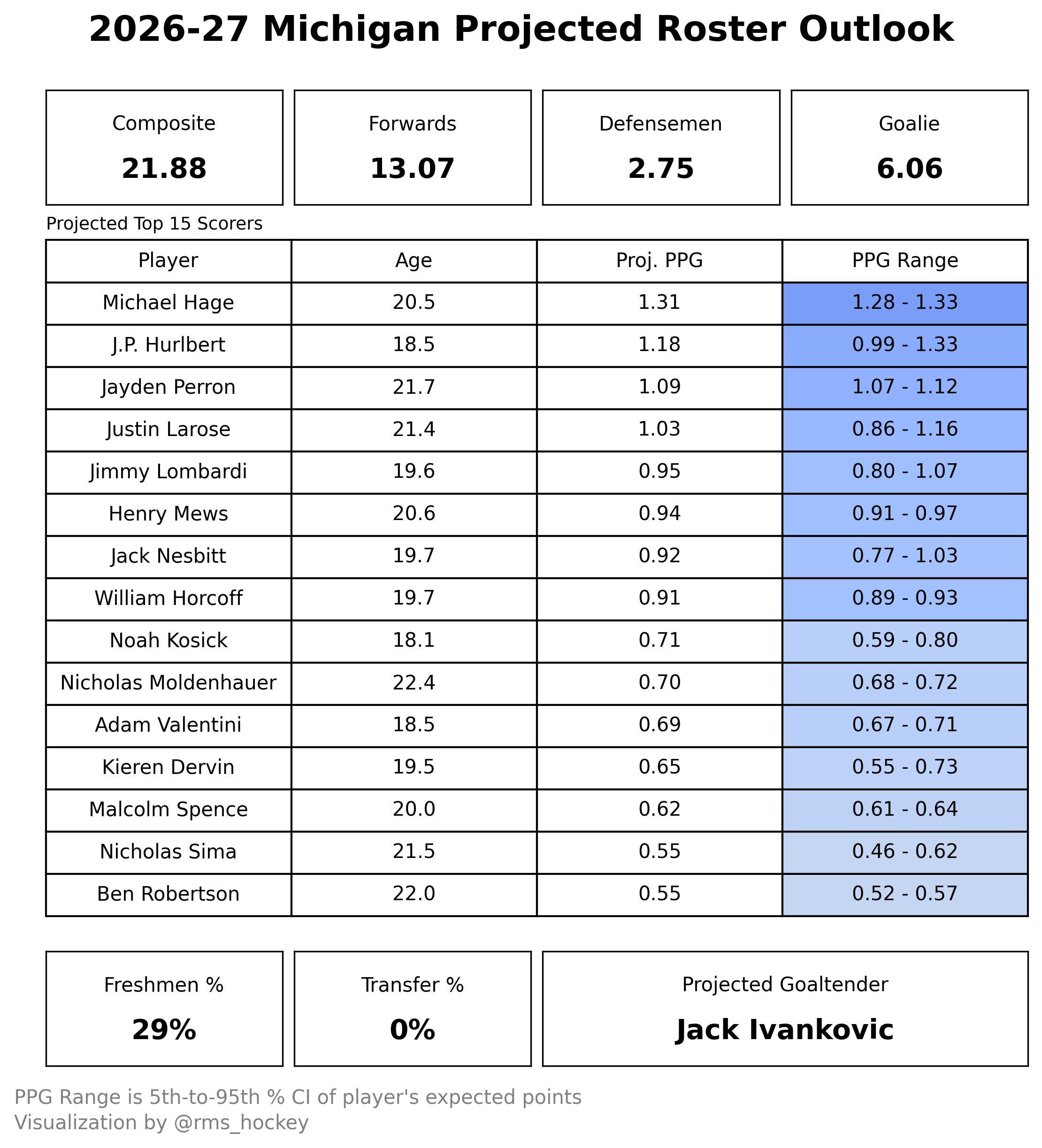
If you are trying to interpret this graphic, please note that it does not suggest Michigan is the 22nd-ranked team. In fact, when compiling preliminary rosters—including outgoing seniors, incoming transfers (which do not apply to Michigan for this particular scenario), and incoming freshmen—the Wolverines are frequently rated as a Top-3 team in the country.

Instead, the graphic indicates that higher ratings for Forwards, Defensemen, and Goalies—and therefore the Composite Team Rating—correlate to better performance.

Regarding player projections, I have listed the Top 15 scorers, their projected age at the start of the 2026–27 season, their mean predicted Points Per Game (PPG), and their PPG range based on the confidence interval (CI).

For example, Michael Hage, who is entering his junior season at Michigan, has a PPG range of 1.28–1.33, resulting in a mean projected PPG of 1.31. This suggests the model is highly confident in this estimate. Conversely, for an incoming freshman like J.P. Hurlbert, who has a PPG range of 0.99–1.33, there is greater variance and less confidence in the point projection.

What Comes Next

This model is not a crystal ball. It does not account for undisclosed injuries, line shuffles, or the random bounces that shape an individual season. What it does is give every skater and every goalie in college hockey a defensible starting point.

With 2026-27 rosters taking shape, projections will begin to roll out this summer, both here and on Twitter/X. Team and conference breakdowns will follow, covering the full picture from incoming freshmen to proven returners, portal transfers, and the goalies behind them.

More to come. Thanks for reading.

— Ryan